The EKV MOSFET Transistor Small-signal Model

The Terminal Charges, Intrinsic Capacitances and Transcapacitances (Version 1)

Abstract

This notebook presents the derivation of the equivalent quasi-static (QS) small-signal circuit. This circuit extends the DC small-signal circuit including the transconductances to high frequency by adding the intrinsic capacitances and transcapacitances.

Licensing

This document is licensed under the Creative Commons License CC BY-NC-SA

1 Introduction

This notebook presents the derivation of the equivalent quasi-static (QS) small-signal circuit. This circuit extends the DC small-signal circuit including the transconductances to high frequency by adding the intrinsic capacitances and transcapacitances. In [1], we have derived this circuit from the non-quasi-static (NQS) model. This approach is rather complex, reason why in this notebook we will derive the QS model in a more standard way using the partitioning of the inversion channel charge between source and drain using the approach proposed by Ward and Dutton [2].

We start expressing the AC charging currents in terms of the intrinsic capacitances modeling the change of charges in the channel, on the gate terminal and depletion capacitance. The Ward and Dutton approach associates a charge to each terminal. The charge on the gate is easy to identify since it is equal to the total inversion charge in the channel and the fixed charges in the depletion capacitance. The charges associated to the source and drain terminals is a bit more tricky to define, but can be defined by partitioning the inversion charge in the channel between the source and the drain following the approach proposed by Ward and Dutton [2].

We then derive the terminal charges and express them in terms of the slope factor \(n\), the normalized charges \(q_s\) and \(q_d\) at the source and drain. We then compute the derivatives with respect to the terminal voltages. We then derive the expressions of all the intrinsic capacitances in terms of \(n\), \(q_s\) and \(q_d\). Finally, we will derive an equivalent small-signal circuit that requires 5 capacitances and 3 transcapacitances.

2 Small-signal AC terminal charging currents

In this section we follow the small-signal model derivation done in [3] [4].

Figure 1: Definition of the voltages and currents [3] [4].

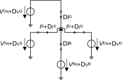
The MOSFET being a four terminal device, we can define the terminal voltages and currents as shown in Figure 1, where \(V_{Dq}\), \(V_{Gq}\), \(V_{Sq}\) and \(V_{Bq}\) are the DC operating point voltages and \(\Delta V_D\), \(\Delta V_G\), \(\Delta V_S\) and \(\Delta V_B\) are the small-signal voltage variations. \(I_D = -I_S\) are the drain and source quiescent currents and \(\Delta I_D\), \(\Delta I_G\), \(\Delta I_S\) and \(\Delta I_B\) are the small-signal variations. Of course the currents need to satisfy the KCL. Neglecting the DC parts and considering only the AC components we can then write \[\begin{equation} \Delta I_D + \Delta I_G + \Delta I_S + \Delta I_B = 0. \end{equation}\] The small-signal source and drain current variations include the change of DC current through the transconductances and the AC components due to the charging currents \[\begin{align} \Delta I_D &= \Delta I_{D,dc} + \Delta I_{D,ac},\\ \Delta I_S &= -\Delta I_{D,dc} + \Delta I_{S,ac}, \end{align}\] where \(\Delta I_{D,dc}\) is the current change due to the transconductances and \(\Delta I_{D,ac}\) and \(\Delta I_{S,ac}\) are the AC charging currents due to the changes of charges \(Q_D\) and \(Q_S\) associated to the drain and source terminals.

Knowing that the charge variations only depend on \(\Delta V_{DB}\), \(\Delta V_{GB}\) and \(\Delta V_{SB}\), we can write the \[\begin{align} \Delta V_{DB} &= \Delta V_D - \Delta V_B,\\ \Delta V_{GB} &= \Delta V_G - \Delta V_B,\\ \Delta V_{SB} &= \Delta V_S - \Delta V_B. \end{align}\]

The small-signal terminal charging currents are given by [3] [4] \[\begin{align} \Delta I_{D,ac}(t) &= +C_{DD}\,\frac{d V_D}{dt}-C_{DG}\,\frac{d V_G}{dt}-C_{DS}\,\frac{d V_S}{dt}-C_{DB}\,\frac{d V_B}{dt},\\ \Delta I_G(t) &= -C_{GD}\,\frac{d V_D}{dt}+C_{GG}\,\frac{d V_G}{dt}-C_{GS}\,\frac{d V_S}{dt}-C_{GB}\,\frac{d V_B}{dt},\\ \Delta I_{S,ac}(t) &= -C_{SD}\,\frac{d V_D}{dt}-C_{SG}\,\frac{d V_G}{dt}+C_{SS}\,\frac{d V_S}{dt}-C_{SB}\,\frac{d V_B}{dt}.\\ \Delta I_B(t) &= -C_{BD}\,\frac{d V_D}{dt}-C_{BG}\,\frac{d V_G}{dt}-C_{BS}\,\frac{d V_S}{dt}+C_{BB}\,\frac{dV_B}{dt}, \end{align}\] where the 16 intrinsic capacitances are defined by \[\begin{align}\label{eqn:int_cap_def} C_{KK} &= \left.+\frac{\partial Q_K}{\partial V_K}\right|_{op},\\ C_{KL} &= \left.-\frac{\partial Q_K}{\partial V_L}\right|_{op}. \end{align}\] where \(K\) and \(L\) are the terminals identifiers. Now, the 16 intrinsic capacitances are not independent. Indeed, because of the KCL, it can be shown that [3] [4] \[\begin{align} C_{DD} &= C_{DG} + C_{DS} + C_{DB} = C_{GD} + C_{SD} + C_{BD},\label{eqn:CDD}\\ C_{GG} &= C_{GD} + C_{GS} + C_{GB} = C_{DG} + C_{SG} + C_{BG},\label{eqn:CGG}\\ C_{SS} &= C_{SD} + C_{SG} + C_{SB} = C_{DS} + C_{GS} + C_{BS},\label{eqn:CSS}\\ C_{BB} &= C_{BD} + C_{BG} + C_{BS} = C_{DB} + C_{GB} + C_{SB}.\label{eqn:CBB} \end{align}\]

For a bulk-referenced model like EKV, we have \[\begin{align} V_D &= V_{DB} + V_B,\\ V_G &= V_{GB} + V_B,\\ V_S &= V_{SB} + V_B, \end{align}\] and the small-signal terminal charging currents can then be written as \[\begin{align} \Delta I_{D,ac}(t) &= +C_{DD}\,\frac{d V_{DB}}{dt}-C_{DG}\,\frac{d V_{GB}}{dt}-C_{DS}\,\frac{d V_{SB}}{dt} +(C_{DD}-C_{DG}-C_{DS}-C_{DB})\,\frac{d V_B}{dt},\\ \Delta I_G(t) &= -C_{GD}\,\frac{d V_{DB}}{dt}+C_{GG}\,\frac{d V_{GB}}{dt}-C_{GS}\,\frac{d V_{SB}}{dt} +(-C_{GD}+C_{GG}-C_{GB}-C_{GS})\,\frac{d V_B}{dt},\\ \Delta I_{S,ac}(t) &= -C_{SD}\,\frac{d V_{DB}}{dt}-C_{SG}\,\frac{d V_{GB}}{dt}+C_{SS}\,\frac{d V_{SB}}{dt} +(-C_{SD}-C_{SG}-C_{SB}+C_{SS})\,\frac{d V_B}{dt}.\\ \end{align}\] Now, the last term of the above equations is actually equal to zero, resulting in \[\begin{align} \Delta I_{D,ac}(t) &= +C_{DD}\,\frac{d V_{DB}}{dt}-C_{DG}\,\frac{d V_{GB}}{dt}-C_{DS}\,\frac{d V_{SB}}{dt},\label{eqn:dIDdt1}\\ \Delta I_G(t) &= -C_{GD}\,\frac{d V_{DB}}{dt}+C_{GG}\,\frac{d V_{GB}}{dt}-C_{GS}\,\frac{d V_{SB}}{dt},\label{eqn:dIGdt1}\\ \Delta I_{S,ac}(t) &= -C_{SD}\,\frac{d V_{DB}}{dt}-C_{SG}\,\frac{d V_{GB}}{dt}+C_{SS}\,\frac{d V_{SB}}{dt}.\label{eqn:dISdt1} \end{align}\]

Replacing \(\eqref{eqn:CDD}\) in \(\eqref{eqn:dIDdt1}\), \(\eqref{eqn:CGG}\) in \(\eqref{eqn:dIGdt1}\) and \(\eqref{eqn:CSS}\) in \(\eqref{eqn:dISdt1}\) results in \[\begin{align} \Delta I_{D,ac}(t) &= (C_{BD}+C_{GD}+C_{SD})\,\frac{dV_{DB}}{dt}-C_{DG}\,\frac{dV_{GB}}{dt}-C_{DS}\,\frac{dV_{SB}}{dt},\\ \Delta I_G(t) &= -C_{GD}\,\frac{dV_{DB}}{dt}+(C_{BG}+C_{DG}+C_{SG})\,\frac{dV_{GB}}{dt}-C_{GS}\,\frac{dV_{SB}}{dt},\\ \Delta I_{S,ac}(t) &= -C_{SB}\,\frac{dV_{DB}}{dt}-C_{SG}\,\frac{dV_{GB}}{dt}+(C_{BS}+C_{DS}+C_{GS})\,\frac{dV_{SB}}{dt}. \end{align}\]

Note that the definition of the intrinsic capacitances given by \(\eqref{eqn:int_cap_def}\) use the derivatives of the terminal charges with respect to an external reference. However, the terminal charges depend on \(V_{DB}\), \(V_{GB}\) and \(V_{SB}\). It is easy to show that the derivatives of the terminal charges with respect to the external reference are actually equal to the derivatives with respect to \(V_{DB}\), \(V_{GB}\) and \(V_{SB}\). For example, for \(\partial Q_D/\partial V_G\), we have \[\begin{equation} C_{DG} = \left.-\frac{\partial Q_D}{\partial V_G}\right|_{V_D,V_S,V_B} = \left.-\frac{\partial Q_D}{\partial V_{GB}}\right|_{V_{DB},V_{SB}} \cdot \left.\frac{\partial V_{GB}}{\partial V_G}\right|_{V_B} = \left.-\frac{\partial Q_D}{\partial V_{GB}}\right|_{V_{DB},V_{SB}}. \end{equation}\] We can therefore calculate the intrinsic capacitances by taking the derivatives wrt \(V_{DB}\), \(V_{GB}\) and \(V_{SB}\). The derivatives of the terminal charges are calculated in the next Section.

3 QS Terminal Charges

3.1 Total inversion charge

The total inversion charge in the channel is given by \[\begin{equation} Q_I = W \, \int_0^L Q_i(x)\,dx. \end{equation}\] We can normalize \(Q_I\) as follows \[\begin{equation}\label{eqn:qI1} q_I \triangleq \frac{Q_I}{W\,L\,Q_{spec}} = \int_0^1 q_i(\xi)\,d\xi \end{equation}\] with \(Q_{spec} \triangleq -2 n\,C_{ox}\,U_T\) and \[\begin{equation} W\,L\,Q_{spec} \triangleq -2 n\,W\,L\,C_{ox}\,U_T. \end{equation}\] Similarly to what was done for calculating the drain current, we can perform the integration in the charge domain, remembering that the drain current is given by \[\begin{equation}\label{eqn:id1} i_d = -(2 q_i+1)\,\frac{dq_i}{d\xi}. \end{equation}\] which gives \[\begin{equation} d\xi = -\frac{2 q_i+1}{i_d}\,dq_i. \end{equation}\] Replacing \(d\xi\) in \(\eqref{eqn:qI1}\) results in \[\begin{equation} q_I = \frac{1}{i_d}\,\int_{q_d}^{q_s} q_i\,(2 q_i+1)\,dq_i, \end{equation}\] where \(q_s \triangleq q_i(\xi=0)\) and \(q_d \triangleq q_i(\xi=1)\).

Performing the integration leads to \[\begin{equation} q_I = \frac{4\,q_s^2 + 4\,q_d^2 + 4\,q_s\,q_d + 3\,q_s + 3\,q_d}{6\,i_d}. \end{equation}\] Replacing the normalized drain current given by \[\begin{equation} i_d = (q_s^2+q_s)-(q_d^2+q_d) = q_s\,(q_s+1) - q_s\,(q_d+1) = (q_s-q_d)\,(q_s+q_s+1), \end{equation}\] results in \[\begin{equation}\label{eqn:qI2} \boxed{ q_I = \frac{1}{6}\,\frac{4\,q_s^2 + 4\,q_d^2 + 4\,q_s\,q_d + 3\,q_s + 3\,q_d}{q_s + q_d + 1}. } \end{equation}\]

In saturation (i.e. for \(q_d=0\)) \(q_I\) reduces to \[\begin{equation} q_{I,sat} = \frac{q_s}{6}\,\frac{4\,q_s+3}{(q_s+1)} = \begin{cases} \frac{q_s}{2} & \textsf{in weak inversion ($q_s \ll 1$)},\\ \frac{2}{3}\,q_s & \textsf{in weak inversion ($q_s \gg 1$)}. \end{cases} \end{equation}\]

3.2 Drain and source terminal charges

The total inversion charge needs to be partitioned between the drain and source terminals. Although this partitioning is a tricky question, under the assumption of constant mobility and uniform doping along the channel, the total inversion charge can be partitioned between the drain and source terminals according to the Ward and Dutton partitioning scheme given by [2] [3] [4] \[\begin{align} Q_D &= W \, \int_0^L \frac{x}{L}\,Q_i(x)\,dx,\\ Q_S &= W \, \int_0^L \left(1-\frac{x}{L}\right)\,Q_i(x)\,dx. \end{align}\] or in normalized form \[\begin{align} q_D &\triangleq \frac{Q_D}{W\,L\,Q_{spec}} = \int_0^1 \xi\,q_i(\xi)\,d\xi ,\\ q_S &\triangleq \frac{Q_S}{W\,L\,Q_{spec}} = \int_0^1 (1-\xi)\,q_i(\xi)\,d\xi, \end{align}\] with \(Q_{spec} \triangleq -2 n\,C_{ox}\,U_T\) and \[\begin{equation} W\,L\,Q_{spec} \triangleq -2 n\,W\,L\,C_{ox}\,U_T. \end{equation}\]

Caution

Carefull not to confuse \(q_S\) with \(q_s\) and \(q_D\) with \(q_d\). \(q_s\) corresponds to the value of the normalized inversion charge at the source \(q_s \triangleq q_i(\xi=0)\), whereas \(q_S\) corresponds to the part of the total normalized inversion charge \(q_I\) that is associated to the source terminal. Similarly, \(q_d\) corresponds to the value of the normalized inversion charge at the drain \(q_d \triangleq q_i(\xi=1)\), while \(q_D\) is the part of the total normalized inversion charge that is associated to the drain terminal.

We can integrate \(\eqref{eqn:id1}\) from to source to a position \(x\) (or \(\xi\)) along the channel \[\begin{equation} i_d\,\xi = \int_{q_i}^{q_s} (2 q_i+1)\,dq_i = (q_s^2+q_s)-(q_i^2+q_i) \end{equation}\] resulting in \[\begin{equation} \xi = \frac{(q_s^2+q_s)-(q_i^2+q_i)}{i_d}. \end{equation}\] Replacing the drain current by \(\eqref{eqn:id1}\), results in \[\begin{equation} \xi = \frac{(q_s^2+q_s)-(q_i^2+q_i)}{(q_s^2+q_s)-(q_d^2+q_d)} = \frac{(q_s-q_i)(q_s+q_i+1)}{(q_s-q_d)(q_s+q_d+1)}. \end{equation}\] The normalized drain charge can then be expressed as \[\begin{equation} q_D = \frac{1}{i_d^2}\,\int_{q_d}^{q_s} [(q_s^2+q_s)-(q_i^2+q_i)]\,q_i\,(2 q_i+1)\,dq_i. \end{equation}\] Performing the integration results in \[\begin{equation}\label{eqn:qD} \boxed{ q_D = \frac{1}{60}\,\frac{16\,q_s^3 + 24\,q_d^3 + 32\,q_s^2\,q_d + 48\,q_d^2\,q_s + 25\,q_s^2 + 45\,q_d^2 + 50\,q_s\,q_d + 10\,q_s + 20\,q_d}{q_s + q_d + 1} } \end{equation}\]

In saturation (i.e. for \(q_d=0\)) \(q_D\) reduces to \[\begin{equation} q_{D,sat} = \frac{q_s}{60}\,\frac{16\,q_s^2+25\,q_s+10}{(q_s+1)^2} = \begin{cases} \frac{q_s}{6} & \textsf{in weak inversion ($q_s \ll 1$)},\\ \frac{4}{15}\,q_s & \textsf{in weak inversion ($q_s \gg 1$)}. \end{cases} \end{equation}\]

Proceeding in a similar way for \(q_S\), we get \[\begin{equation}\label{eqn:qS} \boxed{ q_S = \frac{1}{60}\,\frac{16\,q_d^3 + 24\,q_s^3 + 32\,q_d^2\,q_s + 48\,q_s^2\,q_d + 25\,q_d^2 + 45\,q_s^2 + 50\,q_s\,q_d + 10\,q_d + 20\,q_s}{q_s + q_d + 1} } \end{equation}\]

The source terminal charge can of course be obtained from the drain terminal charge using the source-drain symmetry \(q_S(q_s,q_d)=q_D(q_d,q_s)\).

In saturation (i.e. for \(q_d=0\)) \(q_S\) reduces to \[\begin{equation} q_{S,sat} = \frac{q_s}{60}\,\frac{24\,q_s^2+45\,q_s+20}{(q_s+1)^2} = \begin{cases} \frac{q_s}{3} & \textsf{in weak inversion ($q_s \ll 1$)},\\ \frac{2}{5}\,q_s & \textsf{in strong inversion ($q_s \gg 1$)}. \end{cases} \end{equation}\]

We can check that the sum of \(q_D\) and \(q_S\) is equal to the total charge in the channel \(q_I\) \[\begin{equation} q_I = q_D + q_S = \frac{1}{6}\,\frac{4\,q_s^2 + 4\,q_d^2 + 4\,q_s\,q_d + 3\,q_s + 3\,q_d}{q_s + q_d + 1}, \end{equation}\] which as expected corresponds to the results shown in \(\eqref{eqn:qI2}\).

3.3 Bulk terminal charge

The bulk charge is approximately given by [5] [1] \[\begin{equation} Q_B \cong -\Gamma_b\,C_{ox}\,W\,L\,\sqrt{\Psi_0+V_P}-\frac{n-1}{n}\,Q_I \end{equation}\] or in normalized form \[\begin{equation}\label{eqn:qB} \boxed{ q_B \triangleq \frac{Q_B}{-2n\,W\,L\,C_{ox}\,U_T} = \frac{\gamma_b}{2 n}\,\sqrt{\psi_0+v_p} -\frac{n-1}{n}\,q_I, } \end{equation}\] where \[\begin{align} \gamma_b &\triangleq \frac{\Gamma_b}{\sqrt{U_T}},\\ \psi_0 &\triangleq \frac{\Psi_o}{U_T},\\ v_p & \triangleq \frac{V_P}{U_T}. \end{align}\]

3.4 Gate terminal charge

The gate terminal charge is simply obtained by charge conservation \[\begin{equation}\label{eqn:qG} q_G = -q_B-q_I = -q_B-q_S-q_D, \end{equation}\] where we have ignored the fixed charges. We can write \(q_G\) replacing \(q_B\) by \(\eqref{eqn:qB}\), resulting in \[\begin{equation} \boxed{ q_G = -\frac{1}{n}\,\left(\frac{\gamma_b}{2}\,\sqrt{\psi_0+v_p} + q_I\right). } \end{equation}\]

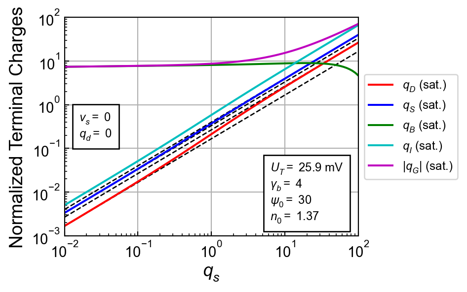
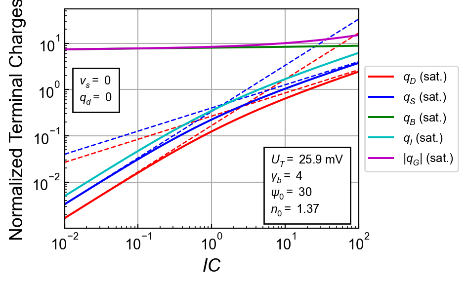
The terminal charges are plotted in saturation (i.e. for q_d=0$) versus \(q_s\) in Figure 2 and versus \(IC\) in Figure 3. We see that the source, drain and total inversion charges are small in weak and moderate and that the bulk charge is dominating. This doesn’t mean that the derivatives of the source, drain and gate terminal charges remain smaller than the derivatives of the bulk terminal charge.

Figure 2: Terminal charges in saturation (\(q_d=0\)) versus \(q_s\) in saturation (\(q_d=0\)).

Figure 3: Terminal charges in saturation (\(q_d=0\)) versus inversion factor \(IC\).

4 Terminal charge derivatives

The purpose of this section is to write the derivatives of the total inversion charge \(q_I\) and the terminal charges \(q_S\), \(q_D\), \(q_B\) and \(q_G\) in terms of \(n\), \(q_s\) and \(q_d\) only. We then need to compute only the derivatives of \(q_I\), \(q_D\) and \(q_S\) wrt \(q_s\) and then get the derivatives of \(q_I\), \(q_D\) and \(q_S\) wrt \(q_d\) by swapping \(q_s\) and \(q_d\) in the obtained derivatives.

Note

To simplify the notation, in the following derivations, \(v_d\), \(v_s\) and \(v_g\) stand actually for \(v_{db} \triangleq V_{DB}/U_T\), \(v_{gb} \triangleq V_{GB}/U_T\) and \(v_{sb} \triangleq V_{SB}/U_T\).

Important

The derivatives of the terminal charges with respect to the terminal voltages will be calculated assuming that the slope factor \(n\) is constant.

4.1 Derivatives of \(q_I\)

The derivatives of \(q_I\) wrt \(v_s\) and \(v_d\) are easy because \(q_I\) depends on \(q_s\) and \(q_d\) where \(q_s\) depends only on \(v_p-v_s\) and not on \(v_d\), whereas \(q_d\) depends only on \(v_p-v_d\) and not on \(v_s\). We can then use the chain rule and express the derivatives of \(q_I\) wrt \(v_d\) and \(v_s\) as \[\begin{align} \frac{\partial q_I}{\partial v_d} &= \frac{\partial q_I}{\partial q_d}\,\left(\frac{d v_d}{d q_d}\right)^{-1},\\ \frac{\partial q_I}{\partial v_s} &= \frac{\partial q_I}{\partial q_s}\,\left(\frac{d v_s}{d q_s}\right)^{-1}. \end{align}\]

Recalling that \(v_p-v_d\) and \(v_p-v_s\) are related to \(q_d\) and \(q_s\) according to \[\begin{align} v_p-v_d &= 2 q_d + \ln(q_d),\\ v_p-v_s &= 2 q_s + \ln(q_s), \end{align}\] we get \[\begin{align} v_d &= v_p - 2 q_d - \ln(q_d),\\ v_s &= v_p - 2 q_s - \ln(q_s), \end{align}\] resulting in \[\begin{align} \frac{d v_d}{d q_d} &= -\frac{2 q_d+1}{q_d},\\ \frac{d v_s}{d q_s} &= -\frac{2 q_s+1}{q_s}. \end{align}\] The derivatives of \(q_I\) wrt \(v_d\) and \(v_s\) then write \[\begin{align} \frac{\partial q_I}{\partial v_d} &= -\frac{q_d}{2 q_d+1}\,\frac{\partial q_I}{\partial q_d} = -\frac{q_d}{6}\,\frac{2\,q_d + 4\,q_d + 3}{(q_s + q_d + 1)^2},\label{eqn:dqIdvd}\\ \frac{\partial q_I}{\partial v_s} &= -\frac{q_s}{2 q_s+1}\,\frac{\partial q_I}{\partial q_s} = -\frac{q_s}{6}\,\frac{2\,q_s + 4\,q_d + 3}{(q_s + q_d + 1)^2}.\label{eqn:dqIdvs} \end{align}\]

When differentiating wrt \(v_g\), we need to account for the fact that both \(q_s\) and \(q_d\) depend on \(v_p\) and therefore on \(v_g\) according to \[\begin{equation} v_p = \frac{v_g-v_{t0}}{n}. \end{equation}\]

The derivative with respect to \(v_g\) can then be written as \[\begin{equation} \frac{d q_I}{d v_g} = \frac{d q_I}{d v_p}\,\frac{d v_p}{d v_g} = \frac{1}{n}\,\frac{d q_I}{d v_p} \end{equation}\] where \[\begin{equation} \frac{d q_I}{d v_p} = \frac{\partial q_I}{\partial q_d}\,\left(\frac{d v_p}{d q_d}\right)^{-1} + \frac{\partial q_I}{\partial q_s}\,\left(\frac{d v_p}{d q_s}\right)^{-1}, \end{equation}\] and \[\begin{align} \frac{d v_p}{d q_d} &= \frac{2 q_d+1}{q_d},\\ \frac{d v_p}{d q_s} &= \frac{2 q_s+1}{q_s}. \end{align}\] The derivative of \(q_I\) wrt \(v_p\) is then given by \[\begin{equation}\label{eqn:dqIdvp} \frac{d q_I}{d v_p} = \frac{1}{6}\,\frac{2\,q_s^2 + 2\,q_d^2 + 8\,q_s\,q_d + 3\,q_s + 3\,q_d}{(q_s + q_d + 1)^2} \end{equation}\] and finally the derivative of \(q_I\) wrt \(v_g\) by \[\begin{equation}\label{dqIdvg} \frac{d q_I}{d v_g} = \frac{1}{6 \, n}\,\frac{2\,q_s^2 + 2\,q_d^2 + 8\,q_s\,q_d + 3\,q_s + 3\,q_d}{(q_s + q_d + 1)^2}. \end{equation}\] Note that the derivative of \(q_I\) wrt \(v_p\) and \(v_g\) are symmetrical with respect to the source and drain. Indeed, we can swap \(q_s\) and \(q_d\) and the expressions \(\eqref{eqn:dqIdvp}\) and \(\eqref{dqIdvg}\) do not change.

4.2 Derivatives of \(q_D\)

Similarly to what was done above for differentiating \(q_I\), the derivatives of \(q_D\) wrt \(v_d\) and \(v_s\) can be expressed as \[\begin{align} \frac{\partial q_D}{\partial v_d} &= \frac{\partial q_D}{\partial q_d}\,\left(\frac{d v_d}{d q_d}\right)^{-1} = -\frac{q_d}{2 q_d+1}\,\frac{\partial q_D}{\partial q_d},\\ \frac{\partial q_D}{\partial v_s} &= \frac{\partial q_D}{\partial q_s}\,\left(\frac{d v_s}{d q_s}\right)^{-1} = -\frac{q_s}{2 q_s+1}\,\frac{\partial q_D}{\partial q_s}. \end{align}\] Performing the differentiation results in \[\begin{align} \frac{\partial q_D}{\partial v_d} &= -\frac{q_d}{30}\,\frac{16\,q_s^2 + 6\,q_d^2 + 18\,q_s\,q_d + 25\,q_s + 15\,q_d + 10}{(q_s + q_d + 1)^3},\\ \frac{\partial q_D}{\partial v_s} &= -\frac{q_s}{30}\,\frac{4\,q_s^2 + 4\,q_d^2 + 12\,q_s\,q_d + 10\,q_s + 10\,q_d + 5}{(q_s + q_d + 1)^3}. \end{align}\]

Note

Notice that the expressions of \(\partial q_D/\partial v_d\) and \(\partial q_D/\partial v_s\) are not symmetrical wrt source and drain.

The derivative of \(q_D\) with respect to \(v_g\) is given by \[\begin{equation} \frac{d q_D}{d v_g} = \frac{d q_D}{d v_p}\,\frac{d v_p}{d v_g} = \frac{1}{n}\,\frac{d q_D}{d v_p}, \end{equation}\] where \[\begin{equation} \frac{d q_D}{d v_p} = \frac{\partial q_D}{\partial q_s}\,\left(\frac{d v_p}{d q_s}\right)^{-1} + \frac{\partial q_D}{\partial q_d}\,\left(\frac{d v_p}{d q_d}\right)^{-1} = \frac{q_s}{2 q_s+1}\,\frac{\partial q_D}{\partial q_s} + \frac{q_d}{2 q_d+1}\,\frac{\partial q_D}{\partial q_d}. \end{equation}\] Performing the differentiation leads to \[\begin{equation} \frac{d q_D}{d v_p} = \frac{1}{30}\,\frac{4\,q_s^3 + 6\,q_d^3 + 28\,q_s^2\,q_d + 22\,q_s\,q_d^2 + 10\,q_s^2 + 15\,q_d^2 + 35\,q_s\,q_d + 5\,q_s + 10\,q_d}{(q_s + q_d + 1)^3} \end{equation}\] and finally \[\begin{equation} \frac{d q_D}{d v_g} = \frac{1}{30\,n}\,\frac{4\,q_s^3 + 6\,q_d^3 + 28\,q_s^2\,q_d + 22\,q_s\,q_d^2 + 10\,q_s^2 + 15\,q_d^2 + 35\,q_s\,q_d + 5\,q_s + 10\,q_d}{(q_s + q_d + 1)^3}. \end{equation}\]

4.3 Derivatives of \(q_S\)

The derivatives of \(q_S\) wrt \(v_d\), \(v_s\) and \(v_g\) are obtained by using the source-drain symmetry, simply swapping \(q_s\) and \(q_d\) in the expressions obtained for the derivatives of \(q_D\). This resuls in \[\begin{align} \frac{\partial q_S}{\partial v_d} &= -\frac{q_d}{30}\,\frac{4\,q_s^2 + 4\,q_d^2 + 12\,q_s\,q_d + 10\,q_s + 10\,q_d + 5}{(q_s + q_d + 1)^3},\\ \frac{\partial q_S}{\partial v_s} &= -\frac{q_s}{30}\,\frac{6\,q_s^2 + 16\,q_d^2 + 18\,q_s\,q_d + 15\,q_s + 25\,q_d + 10}{(q_s + q_d + 1)^3},\\ \frac{d q_S}{d v_g} &= \frac{1}{30\,n}\,\frac{6\,q_s^3 + 4\,q_d^3 + 22\,q_s^2\,q_d + 28\,q_s\,q_d^2 + 15\,q_s^2 + 10\,q_d^2 + 35\,q_s\,q_d + 10\,q_s + 5\,q_d}{(q_s + q_d + 1)^3}. \end{align}\]

4.4 Derivatives of \(q_B\)

The expression \(\eqref{eqn:qB}\) can be rewritten as \[\begin{equation} q_B = q_{B1} + q_{B2}, \end{equation}\] with \[\begin{align} q_{B1} &\triangleq \frac{\gamma_b}{2 n}\,\sqrt{\psi_0+v_p},\label{eqn:qB1}\\ q_{B2} &\triangleq -\frac{n-1}{n}\,q_I.\label{eqn:qB2} \end{align}\] Since \(q_{B1}\) does neither depend on \(v_d\) nor on \(v_s\), we can write the derivatives of \(q_B\) wrt \(v_d\) and \(v_s\) as \[\begin{align} \frac{\partial q_B}{\partial v_d} &= \frac{\partial q_{B2}}{\partial v_d} = -\frac{n-1}{n}\,\frac{\partial q_I}{\partial v_d},\\ \frac{\partial q_B}{\partial v_s} &= \frac{\partial q_{B2}}{\partial v_s} = -\frac{n-1}{n}\,\frac{\partial q_I}{\partial v_s},\label{eqn:dqBdvs} \end{align}\] where \(\partial q_I/\partial v_d\) and \(\partial q_I/\partial v_s\) are given by \(\eqref{eqn:dqIdvd}\) and \(\eqref{eqn:dqIdvs}\), respectively.

From \(\eqref{eqn:qB1}\) and \(\eqref{eqn:qB2}\), we see that both \(q_{B1}\) and \(q_{B2}\) depend on \(v_p\) resulting in \[\begin{align} \frac{\partial q_{B1}}{\partial v_p} &= \frac{\gamma_b}{4n\,\sqrt{\psi_0+v_p}} = \frac{n-1}{2 n},\\ \frac{\partial q_{B2}}{\partial v_p} &= -\frac{n-1}{n}\,\frac{\partial q_I}{\partial v_p}, \end{align}\] since the slope factor \(n\) is defined as \[\begin{equation} n = 1+\frac{\Gamma_b}{2\sqrt{\Psi_0+V_P}} = 1+\frac{\gamma_b}{2\sqrt{\psi_0+v_p}} \end{equation}\] and hence \[\begin{equation} \frac{\gamma_b}{2\sqrt{\psi_0+v_p}} = n-1. \end{equation}\] The derivative of \(q_B\) with respect to \(v_p\) can then be written as \[\begin{equation} \frac{\partial q_B}{\partial v_p} = \frac{n-1}{n}\,\left(\frac{1}{2}-\frac{\partial q_I}{\partial v_p}\right), \end{equation}\] where \(\partial q_I/\partial v_p\) is given by \(\eqref{eqn:dqIdvp}\).

The derivative of \(q_B\) wrt \(v_g\) is finally given by \[\begin{equation} \frac{\partial q_B}{\partial v_g} = \frac{1}{n}\,\frac{\partial q_B}{\partial v_p} = \frac{n-1}{n^2}\,\left(\frac{1}{2}-\frac{\partial q_I}{\partial v_p}\right) \end{equation}\]

4.5 Derivative of \(q_G\)

Recalling that by charge conservation we have \[\begin{equation} q_G = -q_B-q_I. \end{equation}\] Replacing \(q_B\) by \(\eqref{eqn:qB2}\) we get \[\begin{equation}\label{eqn:qG2} q_G = -\frac{\gamma_b}{2 n}\,\sqrt{\psi_0+v_p} +\frac{n-1}{n}\,q_I - q_I = -\frac{1}{n}\,\left(\frac{\gamma_b}{2}\,\sqrt{\psi_0+v_p} + q_I\right). \end{equation}\] The derivative of \(q_G\) wrt \(v_d\) and \(v_s\) are simply \[\begin{align} \frac{\partial q_G}{\partial v_d} &= -\frac{1}{n}\,\frac{\partial q_I}{\partial v_d},\\ \frac{\partial q_G}{\partial v_s} &= -\frac{1}{n}\,\frac{\partial q_I}{\partial v_s}, \end{align}\] where \(\partial q_I/\partial v_d\) and \(\partial q_I/\partial v_s\) are given by \(\eqref{eqn:dqIdvd}\) and \(\eqref{eqn:dqIdvs}\), respectively.

The derivative of \(q_G\) wrt \(v_p\) is given by \[\begin{equation} \frac{\partial q_G}{\partial v_p} = -\frac{\partial q_B}{\partial v_p} - \frac{\partial q_I}{\partial v_p} = -\frac{1}{n}\,\left(\frac{n-1}{2} + \frac{\partial q_I}{\partial v_p}\right), \end{equation}\] where \(\partial q_I/\partial v_p\) is given by \(\eqref{eqn:dqIdvp}\).

The derivative of \(q_G\) wrt \(v_g\) is finally given by \[\begin{equation} \frac{\partial q_G}{\partial v_g} = -\frac{1}{n^2}\,\left(\frac{n-1}{2} + \frac{\partial q_I}{\partial v_p}\right). \end{equation}\]

5 Intrinsic capacitances

5.1 Definition

Note

A capacitance is controlled by the voltage across it while a transcapacitance is modelled by a VCCS controlled by the time derivative of a voltage that is not accross the VCCS. In the following, we will not distinguish between capacitances and transcapacitances. We will only be talking about capacitances.

The definition of the intrinsic capacitances are given in \(\eqref{eqn:int_cap_def}\), which is repeated below for convenience \[\begin{align} C_{KK} &= \left.+\frac{\partial Q_K}{\partial V_K}\right|_{op} = \left.+\frac{\partial Q_K}{\partial V_{KB}}\right|_{op},\\ C_{KL} &= \left.-\frac{\partial Q_K}{\partial V_L}\right|_{op} = \left.-\frac{\partial Q_L}{\partial V_{LB}}\right|_{op}, \end{align}\] with \(K=D,G,S,B\) and \(L=D,G,S,B\).

To keep the consistency with the results obtained by Bucher [5], we normalize the capacitance to \(W\,L\,C_{ox}\), leading to \[\begin{align} c_{kk} &\triangleq \frac{C_{KK}}{W\,L\,C_{ox}} = \left.-2 n\,\frac{\partial q_K}{\partial v_k}\right|_{op},\\ c_{kl} &\triangleq \frac{C_{KL}}{W\,L\,C_{ox}} = \left.+2 n\,\frac{\partial q_K}{\partial v_l}\right|_{op}. \end{align}\]

Note

Notice that the signs have changed because of the original negative normalization parameter \(-2 n\,W\,L\,C_{ox}\,U_T\) used for the terminal charges.

Note

We use small letters for the normalized capacitances and their subscripts to make the notation a bit lighter.

5.2 Charge conservation

From the charge conservation \[\begin{equation} q_G = -q_B - q_I = -q_B - q_S - q_D \end{equation}\] we can write \[\begin{align} \frac{\partial q_G}{\partial v_d} &= -\frac{\partial q_B}{\partial v_d} - \frac{\partial q_S}{\partial v_d} - \frac{\partial q_D}{\partial v_d},\\ \frac{\partial q_G}{\partial v_g} &= -\frac{\partial q_B}{\partial v_g} - \frac{\partial q_S}{\partial v_g} - \frac{\partial q_D}{\partial v_g},\\ \frac{\partial q_G}{\partial v_s} &= -\frac{\partial q_B}{\partial v_s} - \frac{\partial q_S}{\partial v_s} - \frac{\partial q_D}{\partial v_s},\\ \frac{\partial q_G}{\partial v_b} &= -\frac{\partial q_B}{\partial v_b} - \frac{\partial q_S}{\partial v_b} - \frac{\partial q_D}{\partial v_b}. \end{align}\] From the definitions of the normalized capacitances this translates into \[\begin{align} c_{gd} &= -c_{bd} - c_{sd} + c_{dd},\\ -c_{gg} &= -c_{bg} - c_{sg} - c_{dg},\\ c_{gs} &= -c_{bs} + c_{ss} - c_{ds},\\ c_{gb} &= c_{bb} - c_{sb} - c_{db}. \end{align}\] or \[\begin{align} c_{dd} &= c_{gd} + c_{sd} + c_{bd},\\ c_{gg} &= c_{dg} + c_{sg} + c_{bg},\\ c_{ss} &= c_{ds} + c_{gs} + c_{bs},\\ c_{bb} &= c_{db} + c_{gb} + c_{sb} \end{align}\]

5.3 Basic relations between capacitances

5.3.1 Bulk-gate “symmetry”

From \(\eqref{eqn:qG2}\), we have \[\begin{equation} \frac{\partial q_G}{\partial v_s} = -\frac{1}{n}\,\frac{\partial q_I}{\partial v_s}. \end{equation}\] On the other hand from \(\eqref{eqn:dqBdvs}\) we have \[\begin{equation} \frac{\partial q_B}{\partial v_s} = -\frac{n-1}{n}\,\frac{\partial q_I}{\partial v_s} = (n-1)\,\frac{\partial q_G}{\partial v_s}. \end{equation}\] By symmetry we also have \[\begin{equation} \frac{\partial q_B}{\partial v_d} = (n-1)\,\frac{\partial q_G}{\partial v_d}. \end{equation}\] This leads to the following relations between capacitances \[\begin{align} c_{bd} &= (n-1)\,c_{gd},\\ c_{bs} &= (n-1)\,c_{gs}. \end{align}\] Similarly we also have \[\begin{align} c_{db} &= (n-1)\,c_{dg},\\ c_{sb} &= (n-1)\,c_{sg}. \end{align}\]

The derivative of \(q_B\) with respect to \(v_p\) can be written as \[\begin{equation} \frac{\partial q_B}{\partial v_p} = \frac{n-1}{n}\,\left(\frac{1}{2}-\frac{\partial q_I}{\partial v_p}\right) = \frac{n-1}{n}\,\left(\frac{1}{2}-\frac{\partial q_D}{\partial v_p}-\frac{\partial q_S}{\partial v_p}\right) \end{equation}\] This translates into a relation between \(c_{bg}\), \(c_{dg}\) and \(c_{sg}\) \[\begin{equation}\label{eqn:cbg} c_{bg} = \frac{n-1}{n}\,(1-c_{dg}-c_{sg}). \end{equation}\]

From \(\eqref{eqn:qG}\), it is easy to show that \[\begin{equation} c_{gg} = c_{bg} + c_{sg} + c_{dg}. \end{equation}\] Replacing \(c_{bg}\) by \(\eqref{eqn:cbg}\) results in \[\begin{equation} c_{gg} = \frac{1}{n}\,(n-1+c_{dg}+c_{sg}). \end{equation}\]

We also can show that \[\begin{align} c_{dg} &= \frac{c_{dd} - c_{ds}}{n},\\ c_{sg} &= \frac{c_{ss} - c_{sd}}{n}. \end{align}\]

We finally have the following relations \[\begin{align} c_{bd} &= (n-1)\,c_{gd},\label{eqn:cap_rel1}\\ c_{bs} &= (n-1)\,c_{gs},\label{eqn:cap_rel2}\\ c_{db} &= (n-1)\,c_{dg},\label{eqn:cap_rel3}\\ c_{sb} &= (n-1)\,c_{sg},\label{eqn:cap_rel4}\\ c_{bg} &= \frac{n-1}{n}\,(1-c_{dg}-c_{sg}),\label{eqn:cap_rel5}\\ c_{gb} &= c_{bg},\label{eqn:cap_rel6}\\ c_{gg} &= \frac{1}{n}\,(n-1+c_{dg}+c_{sg}),\label{eqn:cap_rel7}\\ c_{dg} &= \frac{c_{dd} - c_{ds}}{n},\label{eqn:cap_rel8}\\ c_{sg} &= \frac{c_{ss} - c_{sd}}{n},\label{eqn:cap_rel9}\\ c_{bb} &= c_{db} + c_{gb} + c_{sb}.\label{eqn:cap_rel10} \end{align}\]

5.4 Primary intrinsic capacitances

We can choose the following 6 capacitances \(c_{gs}\), \(c_{ds}\), \(c_{ss}\), \(c_{gd}\), \(c_{sd}\) and \(c_{dd}\) as primary capacitances and express the other 10 capacitances in terms of these 6 capacitances using \(\eqref{eqn:cap_rel1}\) to \(\eqref{eqn:cap_rel10}\). Additionally, we can use the soure-drain symmetry to express \(c_{gd}\) in terms of \(c_{gs}\), \(c_{sd}\) in terms of \(c_{ss}\) and \(c_{dd}\) in terms of \(c_{ds}\) by swapping \(q_s\) and \(q_d\). We therefore need only to evaluate \(c_{gs}\), \(c_{ds}\) and \(c_{ss}\) which are given below \[\begin{align} c_{gs}(q_s,q_d) &= \frac{q_s}{3}\,\frac{4\,q_d + 2\,q_s + 3}{(q_s + q_d + 1)^2},\\ c_{ds}(q_s,q_d) &= -\frac{n}{15}\,q_s\,\frac{4\,q_s^2 + 4\,q_d^2 + 12\,q_s\,q_d + 10\,q_s + 10\,q_d + 5}{(q_s + q_d + 1)^3},\\ c_{ss}(q_s,q_d) &= \frac{n}{15}\,q_s\,\frac{6\,q_s^2 + 16\,q_d^2 + 18\,q_s\,q_d + 15\,q_s + 25\,q_d + 10}{(q_s + q_d + 1)^3}. \end{align}\] \(c_{gd}\), \(c_{sd}\) and \(c_{dd}\) are then given by \[\begin{align} c_{gd}(q_s,q_d) &= c_{gs}(q_d,q_s),\\ c_{sd}(q_s,q_d) &= c_{ds}(q_d,q_s),\\ c_{dd}(q_s,q_d) &= c_{ss}(q_d,q_s). \end{align}\]

We can then complete the capacitances related to the drain and source terminal charges as follows \[\begin{align} c_{dg} &= \frac{c_{dd}-c_{ds}}{n},\\ c_{db} &= (n-1)\,c_{dg},\\ c_{sg} &= \frac{c_{ss}-c_{sd}}{n},\\ c_{sb} &= (n-1)\,c_{sg}. \end{align}\] Note that, since \(c_{dd}\), \(c_{ds}\), \(c_{ss}\) and \(c_{sd}\) are proportional to \(n\), \(c_{dg}\) and \(c_{sg}\) don’t depend on \(n\).

We can then complete evaluating the remaining capacitances related to the gate and bulk terminal charges as \[\begin{align} c_{gg} &= \frac{n-1+c_{gs}+c_{gd}}{n},\\ c_{bg} &= \frac{n-1}{n}\,(1-c_{dg}-c_{sg}),\\ c_{gb} &= c_{bg},\\ c_{bd} &= (n-1)\,c_{gd},\\ c_{bs} &= (n-1)\,c_{gs},\\ c_{bb} &= c_{db}+c_{gb}+c_{sb}. \end{align}\]

All the normalized capacitances are plotted below versus \(v_p\) and \(v_d\).

Figure 4: Normalized intrinsic capacitances related to the gate terminal charge plotted versus \(v_p\) and \(v_d\).

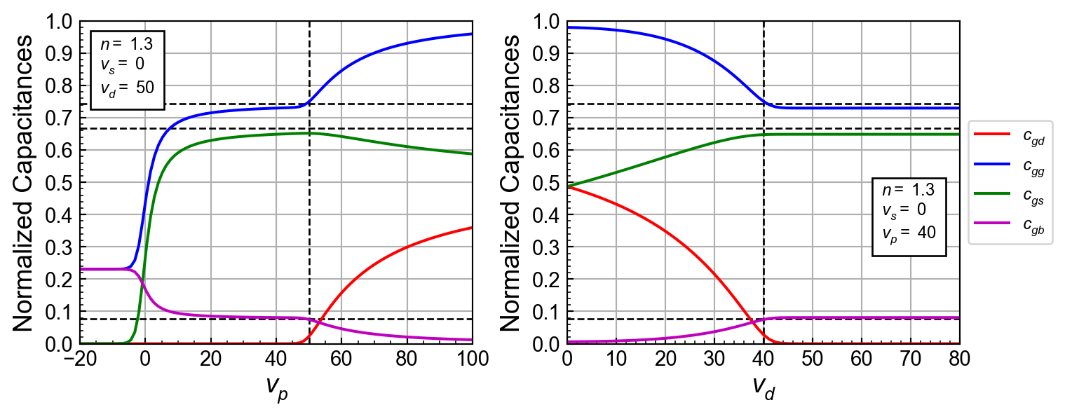
The left plot of Figure 4 shows the four capacitances related to the gate terminal charge versus \(v_p\) for \(v_d =\) 50. \(c_{gd}\) remains zero in saturation and starts to increase when leaving saturation for \(v_p > v_d\). \(c_{gg}\) starts at \((n-1)/n =\) 0.23 and then increases to \(2/3+(n-1)/(3\,n) =\) 0.74 in saturation and finally tends to one when leaving saturation. \(c_{gs}\) starts at zero and increases to 2/3 in strong inversion and saturation and then decreases when leaving saturation for \(v_p > v_d\) to ultimately tend to 0.5. Finally, \(c_{gb}\) starts at \((n-1)/n =\) 0.23 and then decreases to \((n-1)/(3\,n) =\) 0.08 in saturation and finally decreases to zero.

The right plot of Figure 4 shows the same capacitances versus \(v_d\) for \(v_p =\) 40. \(c_{gd}\) starts at 0.5 and tends to zero in saturation for \(v_d > v_p =\) 40. \(c_{gg}\) starts at 1 and decreases to \(2/3+(n-1)/(3\,n) =\) 0.74 in saturation. \(c_{gs}\) starts at 0.5 and increases to reach 2/3 in saturation. Finally \(c_{gb}\) starts at zero and increases to reach \((n-1)/(3\,n) =\) 0.08 in saturation.

Figure 5: Normalized intrinsic capacitances related to the drain terminal charge plotted versus \(v_p\) and \(v_d\).

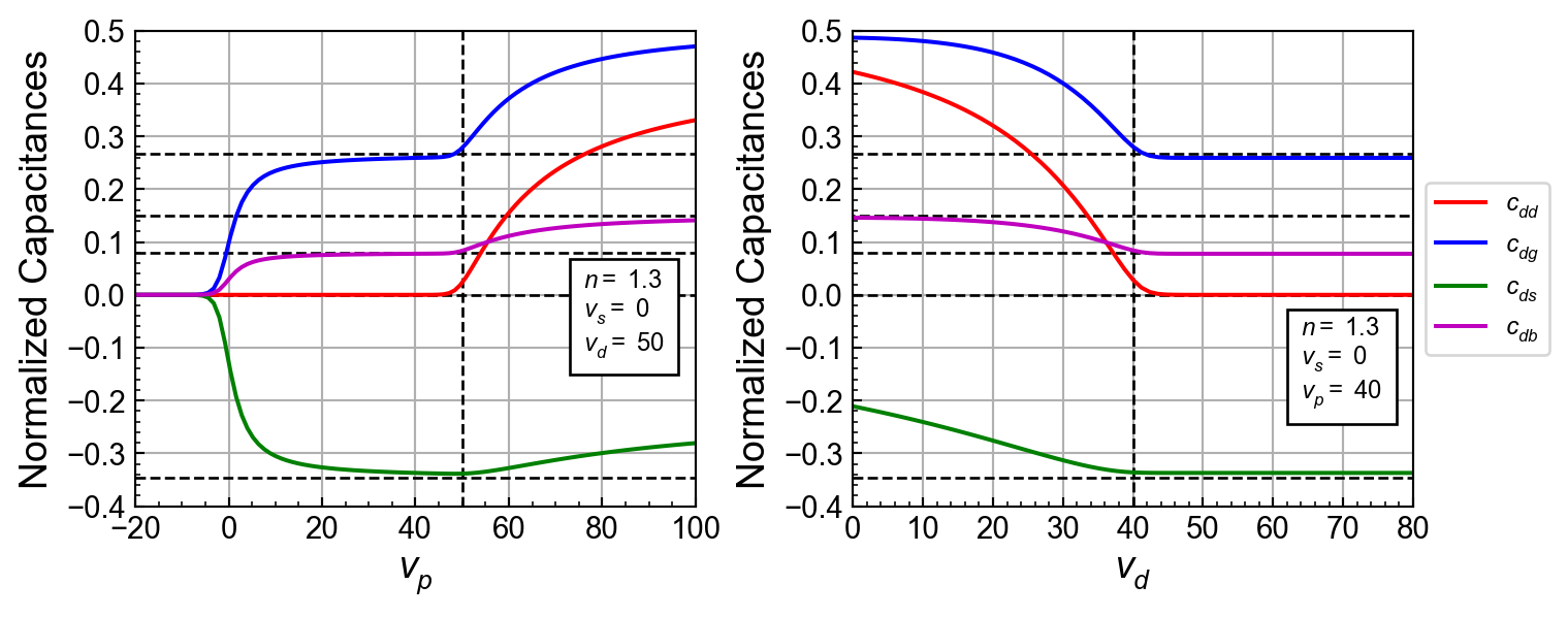
The left plot of Figure 5 shows the four capacitances related to the drain terminal charge versus \(v_p\) for \(v_d =\) 50. \(c_{dd}\) remains zero in saturation and then increases when leaving saturation for \(v_p > v_d =\) 50. \(c_{dg}\) starts at zero and reaches \(4/15 =\) 0.27 in strong inversion and saturation and finally tends to 0.5 when leaving saturation. \(c_{ds}\) starts at zero and becomes equal to \(-4 n/15 =\) -0.35 in strong inversion and saturation. \(c_{db}\) starts at zero and then reaches \(4\,(n-1)/15 =\) 0.08 in strong inversion and saturation and then tends to \((n-1)/2 =\) 0.15 when leaving saturation.

The right plot of Figure 5 shows the same four capacitances versus \(v_d\) for \(v_p =\) 40. \(c_{dd}\) starts at \(n/3 =\) 0.43 and tends to zero in saturation. \(c_{dg}\) starts at 0.5 and tends to \(4/15 =\) 0.27 in saturation. \(c_{ds}\) starts at \(-n/6 =\) -0.22 and tends to \(-4\,n/15 =\) -0.35 in saturation. Finally, \(c_{db}\) starts at \((n-1)/2 =\) 0.15 and tends to \(4\,(n-1)/15 =\) 0.08 in saturation.

Figure 6: Normalized intrinsic capacitances related to the source terminal charge plotted versus \(v_p\) and \(v_d\).

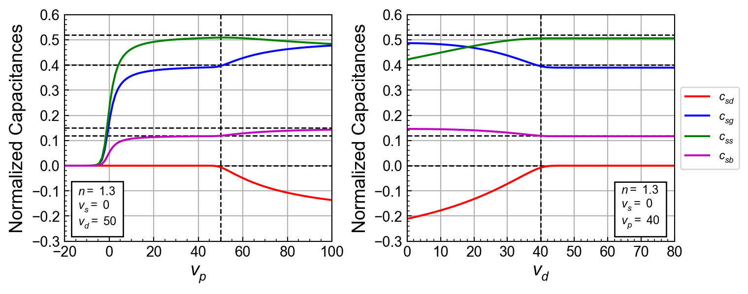
The left plot of Figure 6 shows the four capacitances related to the drain terminal charge versus \(v_p\) for \(v_d =\) 50. \(c_{sd}\) remains zero in strong inversion and saturation and then tends to \(-n/6 =\) -0.22 when leaving saturation. \(c_{sg}\) starts at zero and reaches \(2/5 =\) 0.40 in strong inversion and saturation. \(c_{ss}\) starts at zero and reaches \(2\,n/5 =\) 0.52 in strong inversion and saturation. \(c_{sb}\) starts at zero and then reaches \(2\,(n-1)/5 =\) 0.12 in strong inversion and saturation and then tends to \((n-1)/2 =\) 0.15 when leaving saturation.

The right plot of Figure 6 shows the same four capacitances versus \(v_d\) for \(v_p =\) 40. \(c_{sd}\) starts at \(-n/6 =\) -0.22 and tends to zero in saturation. \(c_{sg}\) starts at 0.5 and tends to \(2/5 =\) 0.40 in saturation. \(c_{ss}\) starts at \(n/3 =\) 0.43 and tends to \(2\,n/5 =\) 0.52 in saturation. Finally, \(c_{sb}\) starts at \((n-1)/2 =\) 0.15 and tends to \(2\,(n-1)/5 =\) 0.12 in saturation.

Figure 7: Normalized intrinsic capacitances related to the bulk terminal charge plotted versus \(v_p\) and \(v_d\).

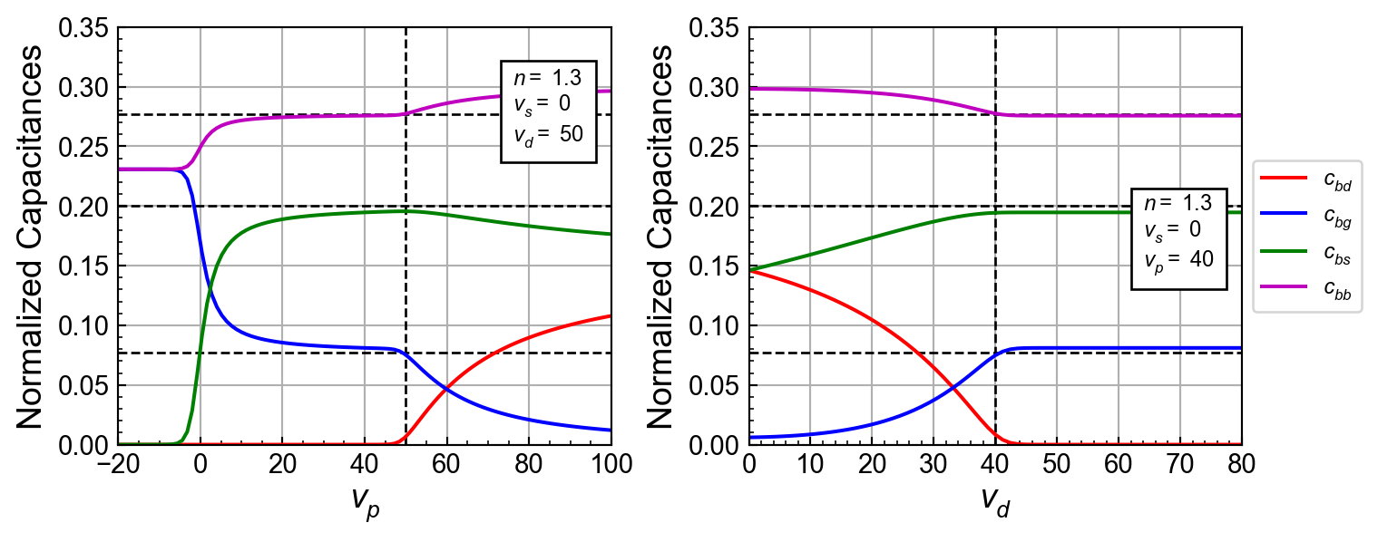
The left plot of Figure 7 shows the four capacitances related to the bulk terminal charge versus \(v_p\) for \(v_d =\) 50. \(c_{bd}\) remains zero in saturation and increases when leaving saturation to tend to \((n-1)/2 =\) 0.15. \(c_{bg}\) starts at \((n-1)/n =\) 0.23 and decreases to \((n-1)/(3\,n) =\) 0.08 in saturation to finally decrease to zero when leaving saturation. \(c_{bs}\) starts at zero and increases to \(2\,(n-1)/3 =\) 0.20 in saturation to decrease to reach \((n-1)/n =\) 0.23. Finally, \(c_{bb}\) starts at \((n-1)/n =\) and reaches \((2\,n-1/n-1)/3 =\) 0.28 in strong inversion and saturation and then tends to \(n-1 =\) 0.30 when leaving saturation.

The right plot of Figure 7 shows the same four capacitances versus \(v_d\) for \(v_p =\) 40. \(c_{bd}\) starts at \((n-1)/2 =\) 0.15 and decreases to reach zero in saturation. \(c_{bg}\) starts at zero and increases to \((n-1)/(3n) =\) 0.08 in saturation. \(c_{bs}\) starts at \((n-1)/n =\) 0.23 and increases to \(2\,(n-1)/3 =\) 0.20 in saturation. Finally, \(c_{bb}\) starts at \(n-1 =\) 0.30 and decreases to \((2\,n-1/n-1)/3 =\) 0.28 in saturation.

Having all the capacitances, we now will map them into a symmetrical and convenient equivalent small-signal circuit.

6 Small-signal equivalent circuit

Figure 8: Equivalent small-signal circuit for the charging currents [6] [7] [1]

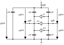
There are many equivalent circuits that can implement the terminal charging currents \(\Delta I_{D,ac}\), \(\Delta I_G\), \(\Delta I_{S,ac}\) and \(\Delta I_B\). In the case of the EKV model, we want to map the charging currents to the small-signal circuit shown in Figure 8 [6] [7] [1], where \[\begin{align} I_m &= -C_m \, \frac{d V_{GB}}{dt},\\ I_{ms} &= -C_{ms} \, \frac{d V_{SB}}{dt},\\ I_{md} &= -C_{md} \, \frac{d V_{DB}}{dt}. \end{align}\]

The terminal charging currents are then given by \[\begin{align} \Delta I_{D,ac}(t) &= -C_{md}\,\frac{dV_{DB}}{dt}-C_m\,\frac{dV_{GB}}{dt}+C_{ms}\,\frac{dV_{SB}}{dt}-C_{gd}\,\frac{dV_{GD}}{dt}+C_{bd}\,\frac{dV_{DB}}{dt},\\ \Delta I_G(t) &= C_{gb}\,\frac{dV_{GB}}{dt}+C_{gs}\,\frac{dV_{GS}}{dt}+C_{gd}\,\frac{dV_{GD}}{dt},\\ \Delta I_{S,ac}(t) &= C_{md}\,\frac{dV_{DB}}{dt}+C_m\,\frac{dV_{GB}}{dt}-C_{ms}\,\frac{dV_{SB}}{dt}-C_{gs}\,\frac{dV_{GS}}{dt}+C_{bs}\,\frac{dV_{SB}}{dt}. \end{align}\] Now \[\begin{align} V_{GS} &= V_{GB}-V_{SB},\\ V_{GD} &= V_{GB}-V_{DB}. \end{align}\] Replacing in the above equations results in \[\begin{align} \Delta I_{D,ac}(t) &= (C_{bd}+C_{gd}-C_{md})\,\frac{dV_{DB}}{dt}-(C_m+C_{gd})\,\frac{dV_{GB}}{dt}+C_{ms}\,\frac{dV_{SB}}{dt},\\ \Delta I_G(t) &= -C_{gd}\,\frac{dV_{DB}}{dt}+(C_{gb}+C_{gd}+C_{gs})\,\frac{dV_{GB}}{dt}-C_{gs}\,\frac{dV_{SB}}{dt},\\ \Delta I_{S,ac}(t) &= C_{md}\,\frac{dV_{DB}}{dt}+(C_m-C_{gs})\,\frac{dV_{GB}}{dt}+(C_{bs}+C_{gs}-C_{ms})\,\frac{dV_{SB}}{dt}. \end{align}\]

In order for the equivalent circuit to produce the same terminal charging currents for the same changes in the terminal voltages, the coefficient of the terminal voltage derivatives must be equal. Equating the coefficients of the drain, gate and source voltage derivatives and solving for \(C_m\), \(C_{ms}\) and \(C_{md}\) results in \[\begin{align} C_m &= C_{dg}-C_{gd},\\ C_{ms} &= -C_{ds},\\ C_{md} &= -C_{sd}. \end{align}\] Notice that the transcapacitances \(C_{ms}\) and \(C_{md}\) are actually positive since \(C_{ds}\) and \(C_{sd}\) are negative.

Similarly for the source terminal current, we get \[\begin{align} C_m &= C_{gs}-C_{sg},\\ C_{ms} &= -C_{ds},\\ C_{md} &= -C_{sd}. \end{align}\]

The values found for \(C_{ms}\) and \(C_{md}\) are identical. However the values for \(C_m\) are different. The equality between the two expressions of \(C_m\) \[\begin{equation} C_m = C_{dg}-C_{gd} = C_{gs}-C_{sg} \end{equation}\] only holds if \(C_{gb}=C_{bg}\) which is actually the case. We can therefore state that the small-signal circuit shown in Figure 8 produces the correct terminal charging currents.

We can now add the transconductances and embed them into the VCCS, giving \[\begin{align} I_m &= Y_m \cdot \Delta V_{GB},\\ I_{ms} &= Y_{ms} \cdot \Delta V_{SB},\\ I_{md} &= Y_{md} \cdot \Delta V_{DB}, \end{align}\] with [1] \[\begin{align} Y_m &= G_m - s\,C_m = G_m\,(1-s\,\tau_{qs}),\\ Y_{ms} &= G_{ms} - s\,C_{ms} = G_{ms}\,(1-s\,\tau_{qs}),\\ Y_{md} &= G_{md} - s\,C_{md} = G_{md}\,(1-s\,\tau_{qs}). \end{align}\] \(\tau_{qs}\) is the quasi-static time constant which is identical for \(Y_m\), \(Y_{ms}\) and \(Y_{md}\) and given by [1] \[\begin{equation} \tau_{qs} = \frac{C_m}{G_m} = \frac{C_{ms}}{G_{ms}} = \frac{C_{md}}{G_{md}}. \end{equation}\] The normalized quasi-static time constant can be expressed in terms of \(q_s\) and \(q_d\) as [1] \[\begin{equation} \frac{\tau_{qs}}{\tau_{spec}} = \frac{\omega_{spec}}{\omega_{qs}} = \frac{1}{30}\,\frac{4\,q_s^2+4\,q_d^2+12\,q_s\,q_d+10\,q_s+10\,q_d+5}{(q_s+q_d+1)^3}, \end{equation}\] where \[\begin{equation}\label{eqn:} \tau_{spec} = \frac{1}{\omega_{spec}} = \frac{L^2}{\mu\,U_T}. \end{equation}\] \(\omega_{qs}\) gives an upper frequency limit for the validity of the QS model. Beyond this limit, the channel behaves more like a non-uniform distributed transmission line and the lumped model of Figure 8 is no more valid. A non-quasi-static (NQS) model is then required [6] [7] [1].

The five intrinsic capacitances of the small-signal circuit of Figure 8 are plotted in Figure 9 and the three transcapacitances are plotted versus \(v_p\) and \(v_d\) in Figure 11.

Figure 9: Normalized intrinsic capacitances of the equivalent small-signal circuit of Figure 8 plotted versus \(v_p\) and \(v_d\).

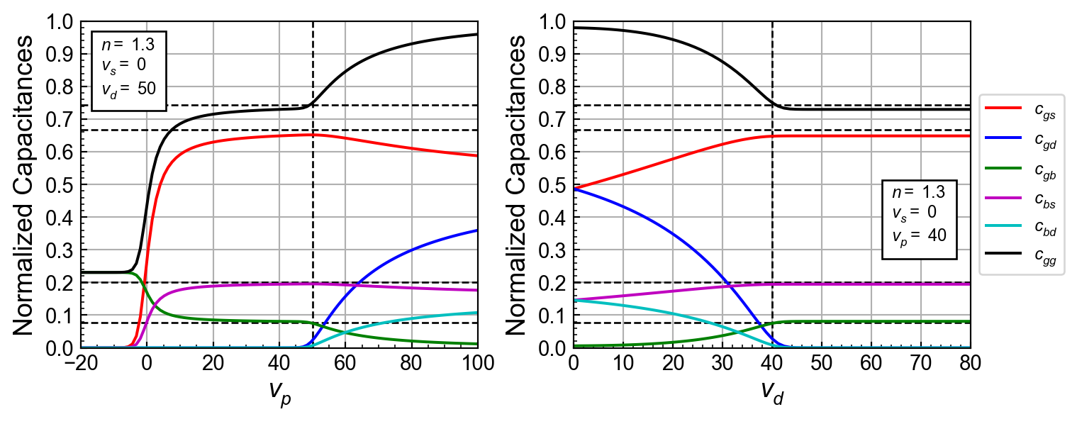
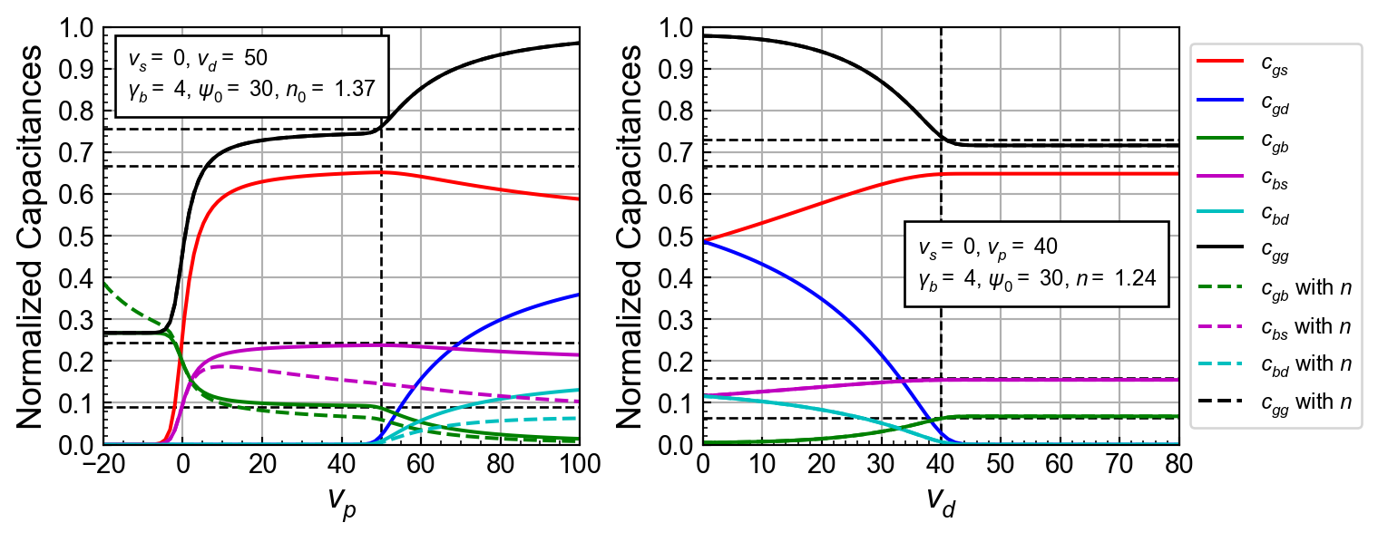
The plots shown in Figure 9 are calculated with a constant slope factor \(n\). This has no impact on \(c_{gs}\) and \(c_{gd}\) since they don’t depend on \(n\). However, \(c_{gb}\), \(c_{bs}\) and \(c_{bd}\) depend \(n\) and are therefore affected by the variation of \(n\) with \(v_p\). This is illustrated in Figure 10 where the dashed lines have been calculated accounting for the dependence of \(n\) to \(v_p\). We see some differences mainly in \(c_{gb}\), \(c_{bs}\), \(c_{bd}\) and \(c_{gg}\). The differences remain small and the approximation of considering \(n\) as constant is sufficient for most purposes.

Figure 10: Normalized intrinsic capacitances of the equivalent small-signal circuit of Figure 8 plotted versus \(v_p\) and \(v_d\) including the dependence of \(n\) with \(v_p\).

Figure 11: Normalized intrinsic transcapacitances of the equivalent small-signal circuit of Figure 8 plotted versus \(v_p\) and \(v_d\).

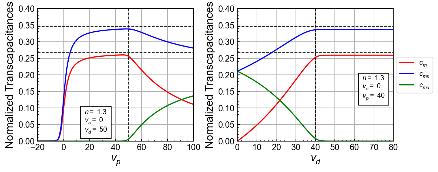
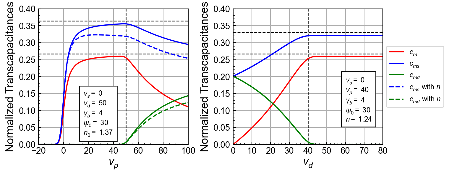
Similarly to the capacitances, the transcapacitances are affected by a change of \(n\) with \(v_p\). Actually, since \(c_{gs}\) and \(c_{sg}\) don’t depend on \(n\), \(c_m\) does not depend on \(n\) neither. However, \(c_{ms}\) and \(c_{md}\) do depend on \(n\) as shown in Figure 12.

Figure 12: Normalized intrinsic transcapacitances of the equivalent small-signal circuit of Figure 8 plotted versus \(v_p\) and \(v_d\) including the dependence of \(n\) with \(v_p\).

7 Conclusion

In this notebook we have derived the high-frequency quasi-static (QS) small-signal model of the intrinsic part of the MOS transistor. We have started by separating the small-signal drain current between a DC part due to the transconductances and an AC part that is due to the charging currents. We have identified the 16 capacitances required to describe the AC small-signal charging currents and shown that they are not all independent and that we actually only need 9 independent capacitances.

The capacitances can be evaluated from the terminal charges. We therefore have derived the four terminal charges under QS assumption. The normalized source and drain terminal charges and the total inversion charge in the channel only depend on \(q_s\) and \(q_d\), while the gate and bulk terminal charges depend on the total inversion charge and on the pinch-off voltage through the parameters \(\gamma_b\) and \(\psi_0\) related to the depletion capacitance.

We then have calculated all the derivatives of the terminal charges wrt to the controling voltages that are required for deriving the capacitances assuming that the slope factor \(n\) remains constant. We have then expressed the derivatives of the normalized terminal charges in terms of \(n\), \(q_s\) and \(q_d\).

We have then used these derivatives to express the normalized intrinsic capacitances in terms of \(n\), \(q_s\) and \(q_d\). We additionnally have derived 10 relations between the various intrinsic capacitances and shown that we only need to know three primary intrinsic capacitances, three others can then be expressed by using the source-drain symmetry by swapping \(q_s\) and \(q_d\) and the other ten can then be expressed by using the 10 capacitance relations.

Finally, we have shown that the charging currents can be mapped into an equivalent small-signal circuit including 5 capacitances and 3 transcapacitances modelled by 3 VCCS which can then be combined with the 3 transcondconductances to obtain the final complete QS small-signal circuit of the intrinsic part of the transistor.

8 References

[1]

C. C. Enz and E. A. Vittoz, Charge-Based MOS Transistor Modeling - The EKV Model for Low-Power and RF IC Design, 1st ed. John Wiley, 2006.

[2]

D. E. Ward and R. W. Dutton, “A Charge-oriented Model for MOS Transistor Capacitances,” IEEE Journal of Solid-State Circuits, vol. 13, no. 5, pp. 703–708, 1978, doi: 10.1109/JSSC.1978.1051123.

[3]

Y. Tsividis, Operation and Modeling of the MOS Transistor, 2nd ed. https://archive.org/details/Operation_And_Modeling_Of_The_Mos_Transistor_Oxford_University_Press_Tsividis_Y/page/n3/mode/2up; Oxford University Press, 2003.

[4]

Y. Tsividis and C. McAndrew, Operation and Modeling of the MOS Transistor, 3rd ed. Oxford University Press, 2011.

[5]

M. Bucher, “Analytical MOS Transistor Modelling for Analog Circuit Simulation,” PhD thesis, EPFL, No. 2114; https://infoscience.epfl.ch/entities/publication/5e5c4962-8077-46ed-ab27-566b31f34aa4, 2000.

[6]

J. M. Sallese and A.-S. Porret, “A Novel Approach to Charge-based Non-Quasi-Static Model of the MOS Transistor Valid in All Modes of Operation,” Solid-State Electronics, vol. 44, no. 6, pp. 887–894, 2000, doi: https://doi.org/10.1016/S0038-1101(00)00040-X.

[7]

A.-S. Porret, J.-M. Sallese, and C. C. Enz, “A Compact Non-quasi-static Extension of a Charge-based MOS Model,” IEEE Transactions on Electron Devices, vol. 48, no. 8, pp. 1647–1654, 2001, doi: 10.1109/16.936582.